Injecting light

Point sources

A point source adds a small current at one cell every step. It is soft: the field there is not overwritten, so waves coming back from your geometry pass straight through it. In a dielectric the current is divided by the local permittivity, the same as a physical current would be.

An array is a set of point sources, each with its own time delay. With element spacing d and steering angle θ, element k is delayed by k · d · sin θ / c.

Plane waves and beams

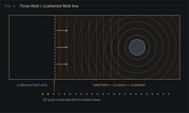
A naive line source radiates in both directions and mixes the incoming wave with everything that comes back. PhotonLab uses a one-sided total-field / scattered-field (TF/SF) line instead:

• A separate one-dimensional FDTD simulation runs alongside the main one and computes the incident wave on its own. It uses the same Courant number, so along an axis its numerical dispersion is identical to the 2D grid. Its far end is terminated with a graded absorbing tail.
• On the line itself, the main grid’s update is corrected with the incident field from the 1D simulation. On one side the main grid then holds the total field; on the other side the incident part cancels exactly, leaving only the scattered field.

In an empty domain nothing leaks into the scattered side: the measured leakage is below 2 × 10⁻⁴ of the incident amplitude in every direction and polarization. That is what makes the reflection measurements in the anti-reflection experiment possible.

The line runs across the whole domain, including the absorbing layer, so a plane wave has no edges to diffract from. A Gaussian beam uses the same mechanism with an amplitude profile exp(−(y − y₀)² / w²) along the line, which places the beam waist on the line.

Waveforms

All waveforms are evaluated at the exact simulation time of each step.

• Continuous: sin(2π f t), multiplied during the first three periods by a raised-cosine ramp. Switching a sine on abruptly would add a burst of unwanted frequencies.
• Pulse: a Ricker wavelet, (1 − 2π²f²τ²) · exp(−π²f²τ²), centred 1.5 periods after the start. It has no DC component, so it does not leave a static charge behind on the grid.
• Wave packet: sin(2π f τ) · exp(−(τ/σ)²) with σ = 2 periods, about six cycles long.