How the solver works

PhotonLab uses the finite-difference time-domain method, introduced by Kane Yee in 1966 and still the workhorse of computational electromagnetics. It does not assume anything about the answer: no rays, no paraxial approximation, no modes. It takes Maxwell’s two curl equations, replaces the derivatives with differences on a grid and steps forward in time.

Two dimensions, two polarizations

The simulation is two-dimensional: nothing changes along the axis that points out of the screen. Maxwell’s equations then split into two independent sets.

TM (the default): the electric field E_z points out of the screen, the magnetic field (H_x, H_y) lies in the plane.
TE: the magnetic field H_z points out of the screen, the electric field (E_x, E_y) lies in the plane.

The colour in the view is the out-of-plane component: E_z in TM, H_z in TE. Which one you need is explained in Polarization and metals.

The Yee grid

The Yee cell: E sits at cell corners, the two H components halfway along the edges

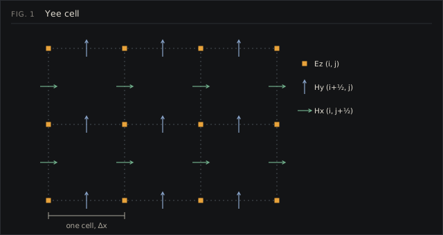
The field components are not stored at the same points. In TM, E_z lives on the grid nodes, H_y halfway between horizontal neighbours and H_x halfway between vertical neighbours. Every spatial derivative then becomes a difference between two neighbours that straddle the point where it is needed, which makes the scheme second-order accurate with no extra work.

In TM the update equations are, with Δx = c = 1:

Hx(i, j+½)  -=  S · [Ez(i, j+1) − Ez(i, j)]
Hy(i+½, j)  +=  S · [Ez(i+1, j) − Ez(i, j)]
Ez(i, j)     =  ca · Ez(i, j) + cb · [Hy(i+½, j) − Hy(i−½, j) − Hx(i, j+½) + Hx(i, j−½)]

ca and cb come from the material at that cell: cb is S/ε, and ca is 1 unless the material is lossy.

The TE equations look exactly the same once you rename the fields (H_z in place of E_z, −E_x and −E_y in place of H_x and H_y) and move the material coefficients from the out-of-plane field to the in-plane ones. PhotonLab uses that symmetry: both polarizations run through the same two loops.

Leapfrog in time

E is updated at whole time steps, H at the half steps in between

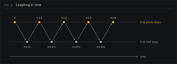
Electric and magnetic fields are also staggered in time. Each step updates H from the current E, then E from the new H. This leapfrog is explicit (no equations to solve) and conserves energy exactly in the absence of losses, which is why a closed box keeps its energy for thousands of steps.

The time step

Explicit schemes are only stable if information does not move more than one cell per step. In 2D the condition is

S = c·Δt / Δx ≤ 1/√2 ≈ 0.707

PhotonLab uses S = 0.5, a comfortable margin that also keeps numerical dispersion low. Light therefore moves half a cell per step.

What one step costs

At 512 × 512 cells a step touches about 260 000 cells, each with a handful of multiply-adds. The loops are written so the compiler can vectorise them with WebAssembly SIMD, and on a recent laptop a step takes around 0.6 ms in the browser. At normal speed the solver runs 640 steps per second on that grid, on a worker thread separate from the interface.