Probes and spectra

Probes

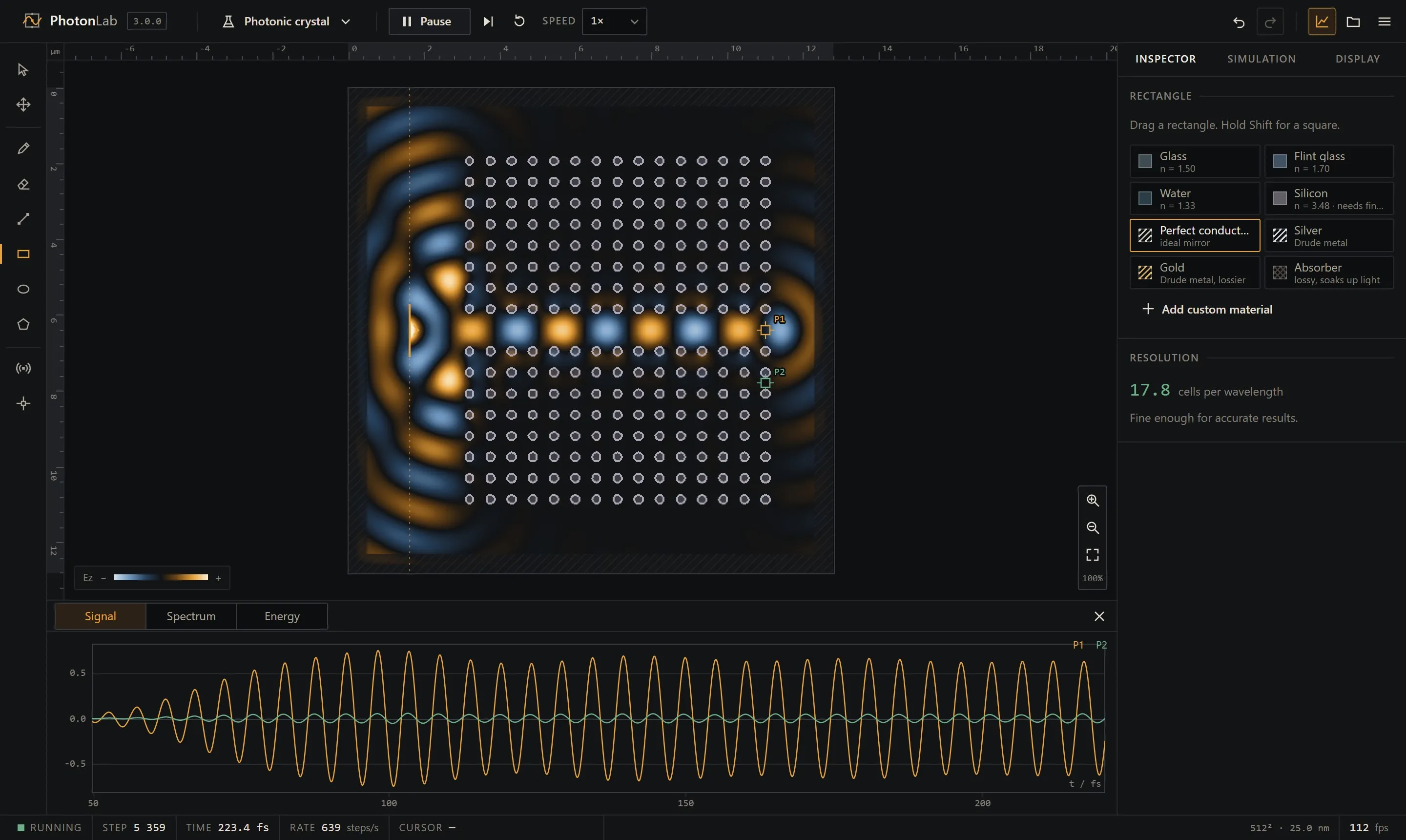
A probe records the field at one point at every time step. Place one with the probe tool (P); a scene can have eight. Each probe gets its own colour, used in every chart.

The probe keeps the last 4096 samples. At the default resolution that is about 170 fs of history, roughly 85 periods of 600 nm light.

In TM mode the probe reads E_z; in TE mode it reads H_z. Both are in normalized units where the incoming plane wave has amplitude 1.

Analysis panel

Open it with A or the chart icon.

Signal. The recorded history of all probes against time in femtoseconds. With a continuous source you can watch the field build up and settle. With a pulse you see the direct pulse first and then each reflection as a separate echo.

Spectrum. The amplitude spectrum of one probe, computed with a Hann-windowed FFT over its history. The horizontal axis is evenly spaced in frequency and labelled in wavelength. The dashed line marks the peak, and its wavelength is printed at the top right. Switch between a linear scale and decibels; dB shows weak components that a linear scale hides.

The frequency resolution is set by the history length: with 4096 samples, neighbouring bins at 600 nm are about 7 nm apart. For a sharp spectrum, let the probe fill its history first.

Energy. The total electromagnetic energy in the domain, ½ Σ (ε E² + H²). In a closed box with mirror walls and no losses it stays flat, which is a good sanity check. With absorbing walls it drops as light leaves.

Exporting probe data

File → Export probe data (CSV) writes one column per probe plus the step number and the time in femtoseconds. The header line records the polarization, cell size and time step, so the file is self-describing for later analysis in Python, MATLAB or a spreadsheet.